
Freight Analysis Framework Version 5 (FAF5) Experimental County-Level Estimates: Technical Report and User Guide
Overview
The Freight Analysis Framework (FAF) database provides estimates of the weight and value of shipments throughout the United States for all commodity types and forms of transportation using a geographic system of 132 FAF zones. The largest zones are entire states. The large zone size limits the useability of FAF for many applications. The user community has expressed a need for more geographically granular commodity flow data to support planning, policymaking, and operational decisions at the state and local levels. In response to this need, BTS developed an experimental county-to-county commodity flow product using publicly available data and transparent methods. This website provides a User Guide and a link to the technical documentation. BTS welcomes users to email FAF@dot.gov with feedback on this experimental product.
Note about Versions
The experimental county-level estimates are based on Freight Analysis Framework version 5.6.1 (FAF5.6.1). The annual estimates have been updated since the county-level release. This page describes differences between FAF5.6.1 and more recent estimates.
Technical Report
Users can download the Technical Report using the link at the top of this webpage.
User Guide
Users can access files for this data release at https://www.bts.gov/faf/county. Data users can download two types of files: state-specific files and disaggregation factors for all counties in the U.S. Table 1 lists the five commodity groups that the release files use to refer to commodity type. The sctgG5 field contains this information. Table 2 lists the mode groups and their codes, which the state-level files use in the dms_mode field. This webpage provides a detailed explanation of these release files. The release files exclude FAF modes 7 and 8.
Table 1. SCTG Group Codes in the Disaggregation Data Products
|
sctgG5 Code |
Definition |
FAF SCTG Code |
|
sctg0109 |
Agricultural products |
1–9 |
|
sctg1014 |
Gravel and mining products |
10–14 |
|
sctg1519 |
Coal and other energy products |
15–19 |
|
sctg2033 |
Chemical, wood and metals |
20–33 |
|
sctg3499 |
Manufactured goods, mixed freight, waste and unknown |
34–99 |
Table 2. New Mode Code in the Disaggregation Factor Tables
|
New Mode Code |
New Mode Definition |
FAF Mode Code |
|
11 |
Truck and Air |
1—Truck 4—Air |
|
2 |
Rail |
2—Rail |
|
3 |
Water |
3—Water |
|
5 |
Multiple modes and mail |
5—Multiple modes and mail |
|
6 |
Pipeline |
6—Pipeline |
STATE-BASED DISAGGREGATION RESULTS
The release includes 51 state-specific zip files (including one zip file for Washington, DC). Each file represents flows using county-level geography for the main state and for states adjacent to the main state. Geographic representation of flows outside of this area consists of FAF zones. Each state zip file contains four tables representing 1) county-level OD flows for the state of interest and every adjacent state, 2) county-to-FAF zone Origin-Destination (OD) flows from the multi-state area to all other FAF zones, 3) FAF zone-to-county OD flows from all other FAF zones to the multi-state area, and 4) FAF zone-to-FAF zone OD flows from all other FAF zones to all other FAF zones.
Example: Release File for the State of Maryland
Figure 1 shows the multi-state area of Maryland and its immediate area, which includes four adjacent states (Pennsylvania, Delaware, Virginia, and West Virginia) and the District of Columbia. The zip file contains:
- Table 1: county-to-county commodity flows between all counties in this multi-state area
- Table 2: county-to-FAF zone commodity flows from counties in the multi-state area to the FAF zones outside of this area
- Table 3: FAF zone-to-county commodity flows from the FAF zones outside of the multi-state area to counties in the multi-state area
- Table 4: FAF zone-to-FAF zone commodity flows between all other FAF zones outside of the multi-state area.
Figure 1. Maryland with Surrounding States and Washington, DC
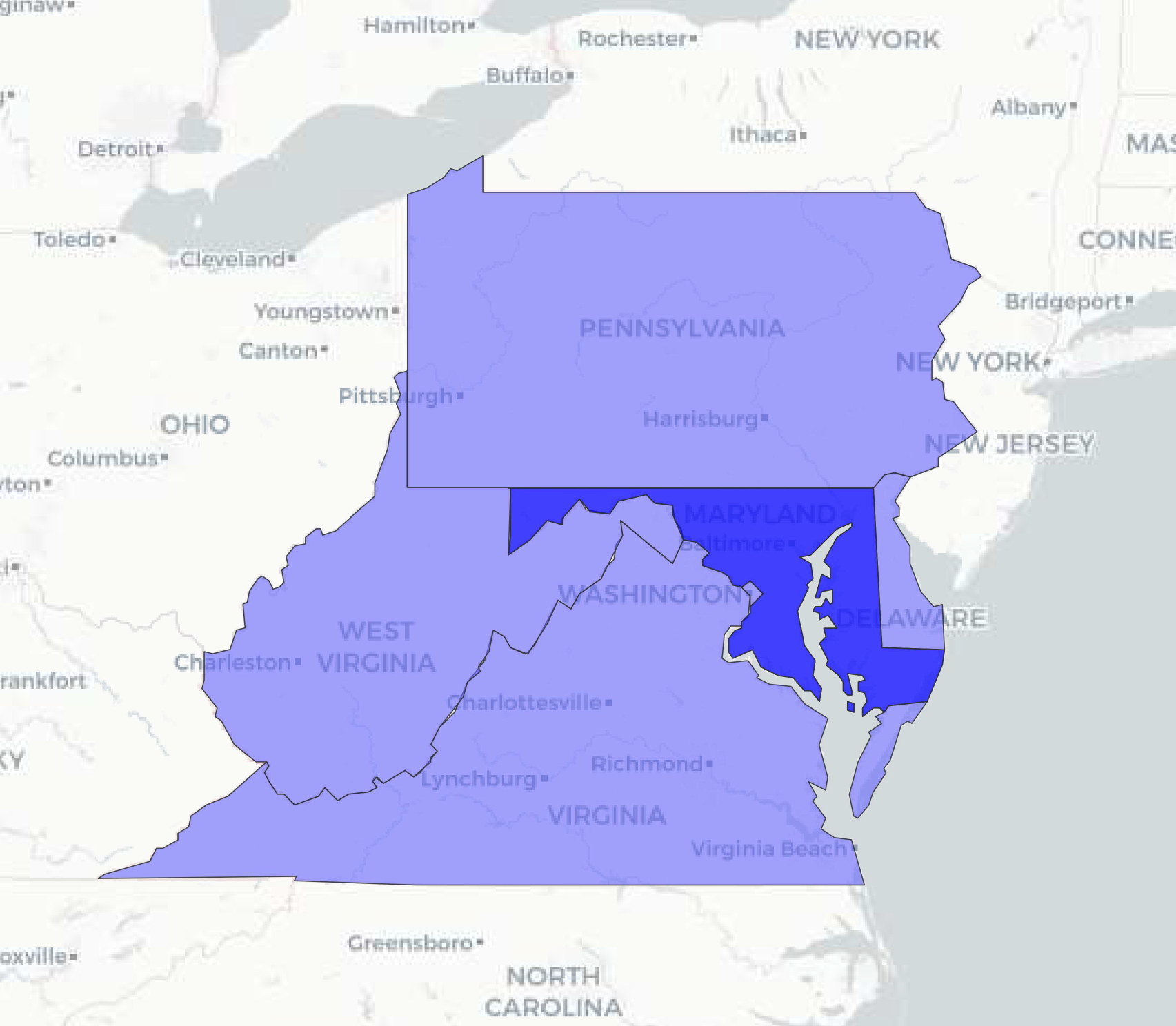
Source: BTS and OpenStreetMap 2024.
DISAGGREGATION FACTORS: DESCRIPTION AND APPLICATION
The full set of county-level factors (origin and destination factors) are contained in one zip file. Users can merge these factors with FAF regional databases to create a county-level database for a customized geographic area or for the entire U.S. Users will need to download the FAF regional databases from www.bts.gov/faf. The FAF database download includes metadata with variable dictionaries. The factors are available for four modes and five commodity groups. The zip file contains files with disaggregation factors for four modes:
- Rail (rail_origin_factors.csv and rail_destination_factors.csv)
- Water (water_origin_factors.csv and water_destination_factors.csv)
- Truck (truck_origin_factors.csv and truck_destination_factors.csv)
- Pipeline (pipeline_origin_factors.csv and pipeline_destination_factors.csv)
Users can apply the truck factors to air and multiple modes and mail modes to generate county-to-county flows for these modes. This experimental product does not include methods to disaggregate flows by other or unknown mode, or flows that use no domestic mode.
Table 3 explains the variables in the origin factor files. The data structure in the destination factor file is the same. The factor files include the county FIPS code, the county’s corresponding FAF zone code, commodity group, and the disaggregation factor for that combination of county and commodity group.
Table 3. Layout of FAF Origin Factor Table
|
Variable name |
Description |
|
dms_orig |
Origin FAF code |
|
dms_orig_cnty |
Origin county FIPS code |
|
sctgG5 |
Commodity group code |
|
f_orig |
The proportion of FAF zone tons of sctgG5 that originate in this county |
Users can apply the process that Figure 2 illustrates to disaggregate FAF zone flows to the county level. The steps are:
- (Optional) Select FAF trips for the area of interest. This will reduce the size of the input dataset, which improves efficiency in the remaining disaggregation steps. For example, to generate county-to-county tonnage estimates only for Iowa to Idaho, the user can select flows with dms_orig=190 and dms_dest=160, filtering out all other flows.
- Select FAF trips for the mode of interest. For example, to disaggregate rail flows, select flows with dms_mode=2 (rail) from the previous step, filtering out all other flows.
- Use the commodity correspondence from Table 1 to summarize the flows from the previous step (red box in Figure 1) using the five commodity groups. This will reduce the 42 commodity categories to five.
- Join the resulting table from the previous step to the origin factor table based on the FAF origin zone (dms_orig) and commodity group (sctgG5) columns. The resulting file now contains the factor for the origin county and commodity group (f_orig).
- Join the resulting table from the previous step to the destination factor table based on the FAF destination zone (dms_dest) and commodity group (sctgG5) columns. The resulting file now contains the factor for the destination county and commodity group (f_dest).
- The resulting table contains all possible combinations of county pairs and commodity groups that are present in the original FAF estimates for the selected area and mode. Users can calculate the final county-to-county tonnage by commodity group by multiplying the total FAF zone-level tons by the origin factor and the destination factor. The Figure 2 note shows these formulas.
Figure 2. Example: Applying Disaggregation Factors
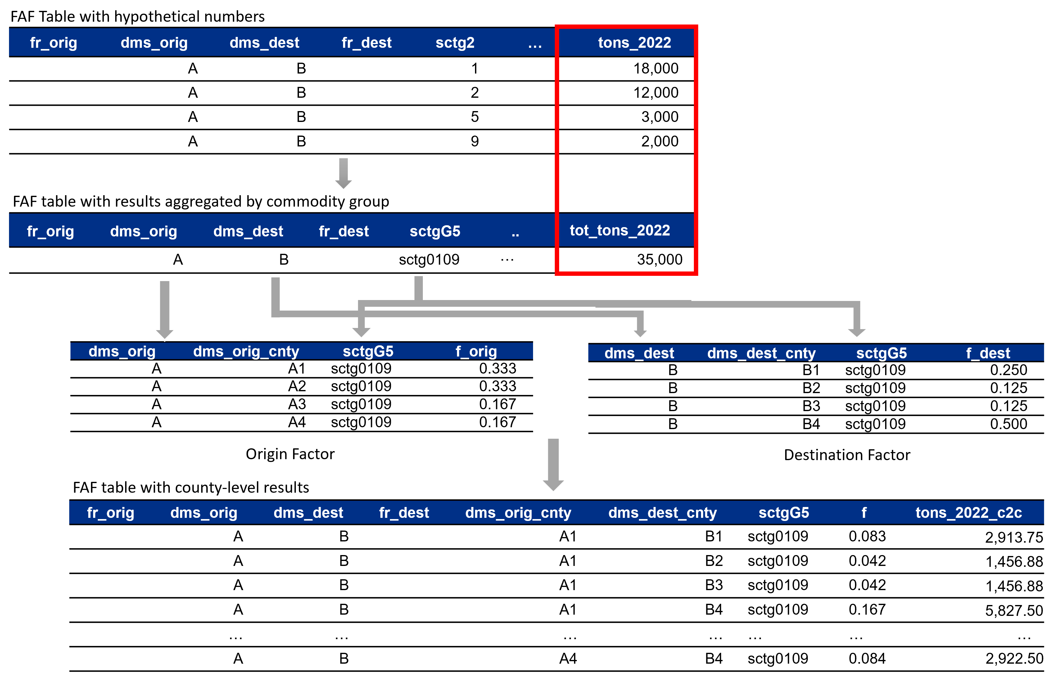
Source: BTS.
Note: f = f_orig*f_dest, tons_2022_c2c = tons_2022*f